
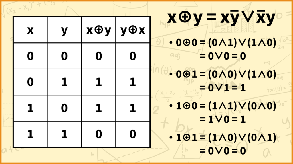
排他的論理和\(\oplus\)は論理変数\(x,\;y\)に対して
\(x \oplus y = x\bar{y} \vee \bar{x}y\)
となる。
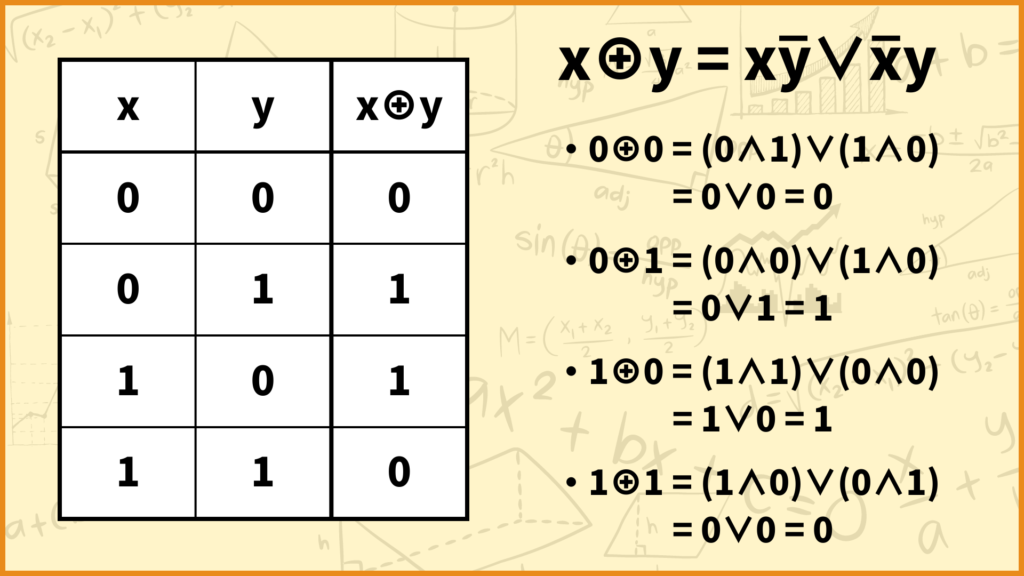
排他的論理和を簡単に説明すると\(x\)と\(y\)の値が一緒のときは0を取り、異なるときは1を取ります。
【Udemy講座公開のお知らせ】
このたびUdemyで数理最適化の講座を公開しました!この講座は「数理最適化を勉強してみたいけど数式が多くて難しい…」という方向けに、どうやって最適化問題を定式化すれば良いかを優しく丁寧に解説しています!
排他的論理和(EXOR)の性質
排他的論理和\(\oplus\)は以下の式が成り立ちます。
1つ目:\(x \oplus y = y \oplus x\)
2つ目:\((x \oplus y) \oplus z = x \oplus (y \oplus z)\)
3つ目:\(x \wedge (y \oplus z) = (x \wedge y) \oplus (x \wedge z)\)
4つ目:\(x \oplus 0 = x\)
5つ目:\(x \oplus 1 = \bar{x}\)
6つ目:\(x \oplus x = 0\)
7つ目:\(x \oplus \bar{x} = 1\)
それぞれ成立するのを確認してみましょう。
排他的論理和(EXOR)の性質を確かめる
1つ目
1つ目:\(x \oplus y = y \oplus x\)
これはすぐにわかりますね。\(x \oplus y = x\bar{y} \vee \bar{x}y = \bar{x}y \vee x\bar{y} = y \oplus x\)なことからも分かります。
この性質は交換律と呼ばれます。
2つ目
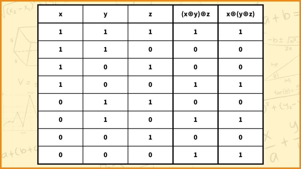
2つ目:\((x \oplus y) \oplus z = x \oplus (y \oplus z)\)
上の表の右側の列2つを計算すると\((x \oplus y) \oplus z = x \oplus (y \oplus z)\)が成り立つのが分かります。
この性質は結合律と呼ばれます。
\((1 \oplus 1) \oplus 1 =0 \oplus 1 = 1\)
\(1 \oplus (1 \oplus 1) =1 \oplus 0 = 1\)
\((1 \oplus 1) \oplus 0 =0 \oplus 0 = 0\)
\(1 \oplus (1 \oplus 0) =1 \oplus 1 = 0\)
\((1 \oplus 0) \oplus 1 =1 \oplus 1 = 0\)
\(1 \oplus (0 \oplus 1) =1 \oplus 1 = 0\)
\((1 \oplus 0) \oplus 0 =1 \oplus 0 = 1\)
\(1 \oplus (0 \oplus 0) =1 \oplus 0 = 1\)
\((0 \oplus 1) \oplus 1 =1 \oplus 1 = 0\)
\(0 \oplus (1 \oplus 1) =0 \oplus 0 = 0\)
\((0 \oplus 1) \oplus 0 =1 \oplus 0 = 1\)
\(0 \oplus (1 \oplus 0) =0 \oplus 1 = 1\)
\((0 \oplus 0) \oplus 1 =0 \oplus 1 = 1\)
\(0 \oplus (0 \oplus 1) =0 \oplus 1 = 1\)
\((0 \oplus 0) \oplus 0 =0 \oplus 0 = 0\)
\(0 \oplus (0 \oplus 0) =0 \oplus 0 = 0\)
3つ目
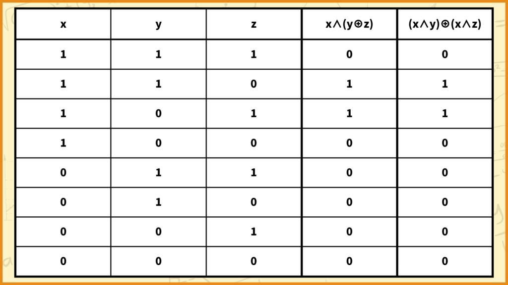
3つ目:\(x \wedge (y \oplus z) = (x \wedge y) \oplus (x \wedge z)\)
上の表の右側の列2つを計算すると\(x \wedge (y \oplus z) = (x \wedge y) \oplus (x \wedge z)\)が成り立つのが分かります。
この性質は分配律と呼ばれます。
\(1 \wedge (1 \oplus 1) = 1 \wedge 0 = 0\)
\((1 \wedge 1) \oplus (1 \wedge 1) = 1 \oplus 1 = 0\)
\(1 \wedge (1 \oplus 0) = 1 \wedge 1 = 1\)
\((1 \wedge 1) \oplus (1 \wedge 0) = 1 \oplus 0 = 1\)
\(1 \wedge (0 \oplus 1) = 1 \wedge 1 = 1\)
\((1 \wedge 0) \oplus (1 \wedge 1) = 0 \oplus 1 = 1\)
\(1 \wedge (0 \oplus 0) = 1 \wedge 0 = 0\)
\((1 \wedge 0) \oplus (1 \wedge 0) = 0 \oplus 0 = 0\)
\(0 \wedge (1 \oplus 1) = 0 \wedge 0 = 0\)
\((0 \wedge 1) \oplus (0 \wedge 1) = 0 \oplus 0 = 0\)
\(0 \wedge (1 \oplus 0) = 0 \wedge 1 = 0\)
\((0 \wedge 1) \oplus (0 \wedge 0) = 0 \oplus 0 = 0\)
\(0 \wedge (0 \oplus 1) = 0 \wedge 1 = 0\)
\((0 \wedge 0) \oplus (0 \wedge 1) = 0 \oplus 0 = 1\)
\(0 \wedge (0 \oplus 0) = 0 \wedge 0 = 0\)
\((0 \wedge 0) \oplus (0 \wedge 0) = 0 \oplus 0 = 0\)
4つ目~7つ目
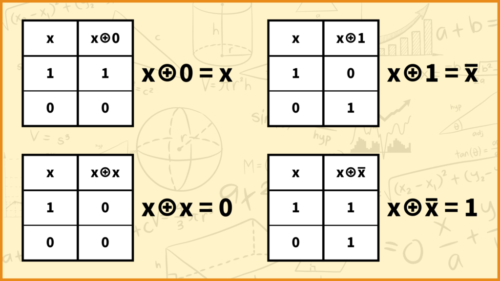
4つ目:\(x \oplus 0 = x\)
5つ目:\(x \oplus 1 = \bar{x}\)
6つ目:\(x \oplus x = 0\)
7つ目:\(x \oplus \bar{x} = 1\)
これも1と0を代入するとすぐに分かりますね。
おわりに
いかがでしたか。
今回の記事では排他的論理和(EXOR)について解説していきました。
今後もこのような論理関数に関する記事を書いていきます!
最後までこの記事を読んでくれてありがとうございました。
普段は統計検定2級の記事を書いてたりします。
ぜひ他の記事も読んでみてください!
このブログの簡単な紹介はこちらに書いてあります。
興味があったら見てみてください。
このブログでは経営工学を勉強している現役理系大学生が、経営工学に関することを色々話していきます!
ぼくが経営工学を勉強している中で感じたことや、興味深かったことを皆さんと共有出来たら良いなと思っています。
そもそも経営工学とは何なのでしょうか。Wikipediaによると
経営工学(けいえいこうがく、英: engineering management)は、人・材料・装置・情報・エネルギーを総合したシステムの設計・改善・確立に関する活動である。そのシステムから得られる結果を明示し、予測し、評価するために、工学的な分析・設計の原理・方法とともに、数学、物理および社会科学の専門知識と経験を利用する。
引用元 : 経営工学 – Wikipedia
長々と書いてありますが、要は経営、経済の課題を理系的な観点から解決する学問です。